Chapter 3 The Shell Model

3.1 Introduction

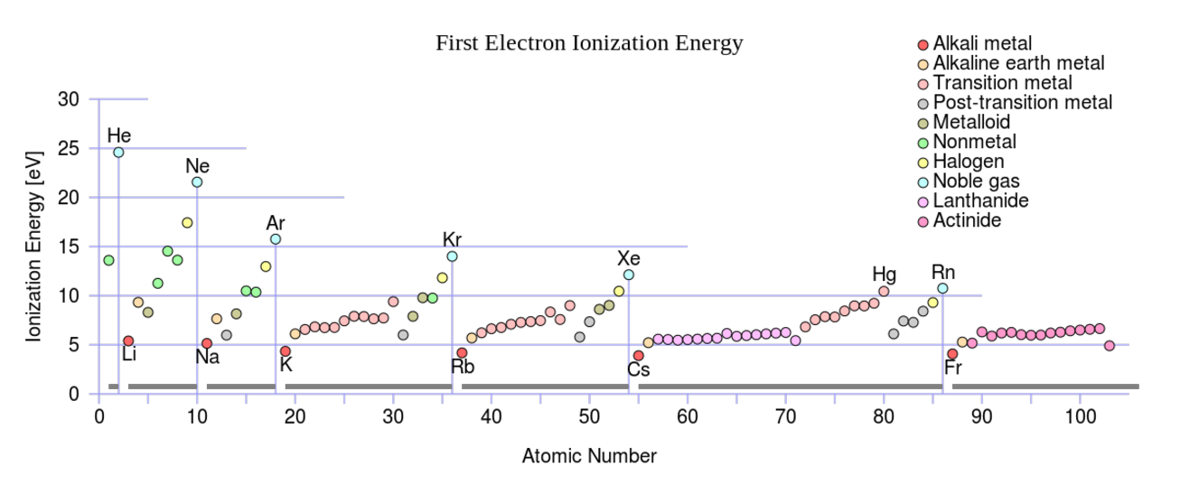
The atomic shell model, in which we successively fill the electronic shells with electrons, has proved remarkably successful in explaining the chemical properties of the elements and the details of atomic structure (see, for example, Fig. 3.1).

Figure 3.1: The ionisation energy of the elements.

A nucleus has similar energy levels. The energy levels are determined by solving the Schrödinger equation for the nuclear potential. However, the rules for filling protons and neutrons are different, so don’t confuse them with electronic energy levels.

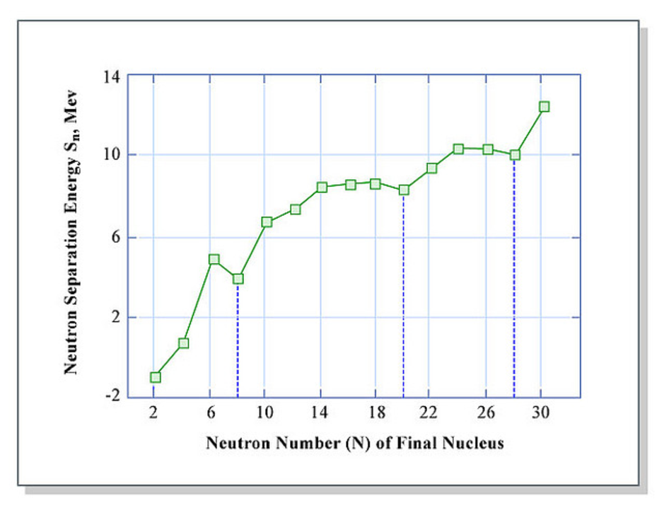
What evidence is there in support of the existence of nuclear energy shells? Separating a neutron from a nucleus is described by the equation

$${}_Z{}^{A}X\to {}_Z{}^{A-1}X+n.$$ (3.1)

The energy required to separate a neutron can be calculated from the mass difference between the initial and final states. This is shown in Fig. 3.2, where the x-axis shows the number of neutrons in the final nucleus. It can be seen that the separation energy is smaller for final nuclei with 8, 20, and 28 neutrons.

Figure 3.2: Neutron separation energies.

Figure 3.3: Two proton (top) and two neutron (bottom) separation energies.

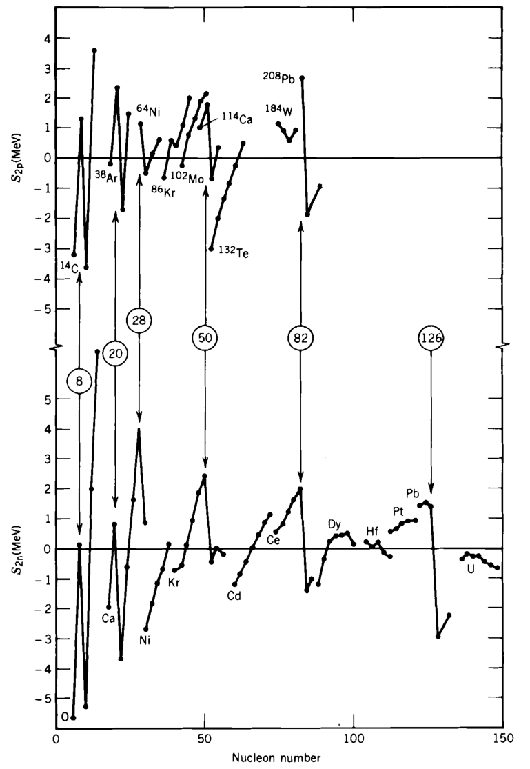
Similar behaviour is observed for two neutron and proton separation energies. Fig. 3.3 shows the energy required to remove two protons (the two-proton separation energy) from a sequence of isotones (nuclei with the same number of neutrons) (top), and two neutrons from a sequence of isotopes (bottom).

The data are plotted as the differences between the measured values and the predictions of the semi-empirical mass formula (see lecture 2), and clearly reveal sharp discontinuities of the separation energies that are very similar to the discontinuities in the atomic ionization energies (Fig. 3.1). Further, these discontinuities occur when we have particular numbers of nucleons, the so-called ‘magic numbers’ where

$$Z\mathrm{or}N=2,8,20,28,50,82,126.$$ (3.2)

These must represent the effects of filled nuclear shells.

3.1.1 Nuclear energy levels

It is therefore tempting to ask whether a similar model to the atom might explain variation in nuclear properties. There are of course differences: in the electronic case, the potential in which the electrons move, and for which we use the Schrodinger equation to determine the energy levels, is supplied by the nucleus, whereas the nucleons move in a potential they themselves generate. The electronic energy levels are associated with spatial orbits in which electrons move freely; this is difficult to envisage for the comparatively bulky nucleons moving in the confines of a small nucleus.

The potential issue is dealt with by considering the motion of a nucleon in a field generated by the others. The issue of orbits depends on the Pauli principle. If two nucleons collide they will exchange energy. But this requires a transfer from a lower lying level to a valence band and this entails more energy than might reasonably be exchanged. So collisions don’t occur and nucleons orbit as if transparent.

Careful 3.1.1.

In the following sections, we will discuss nuclear energy levels and the associated filling rules for protons and nucleons. These are different from the atomic energy levels you will discuss in semester 2, so do not confuse them.

Background 3.1.1 (Quantum Mechanics Angular Momentum).

We require some results from the quantum theory of angular momentum. Classically, the angular momentum $𝐥$ of a particle with momentum $𝐩$ at a position $\mathrm{r}$ is

$$𝐥=𝐫\times 𝐩.$$ (3.3)

To quantise we replace $𝐫$ and $𝐩$ with their operator equivalents, e.g. ${\widehat{p}}_x=-i\mathrm{\hslash }\partial /\partial x$. The components of angular momentum are then of the form ${\widehat{l}}_x=\widehat{y}{\widehat{p}}_z-\widehat{z}{\widehat{p}}_y$.

Since from now on we will always be dealing with quantum mechanical operators we omit the hats. The square of the angular momentum is ${𝐥}^2=l_x^2+l_y^2+l_z^2$. To find its expectation value (denoted by angled brackets) we compute

$$⟨{𝐥}^2⟩=\int {\psi }^{\star }{𝐥}^2\psi ,$$ (3.4)

which is found to be $⟨{𝐥}^2⟩=\mathrm{\ell }(\mathrm{\ell }+1){\mathrm{\hslash }}^2$, where $\mathrm{\ell }$ is the angular momentum quantum number. The z-component of the angular momentum is found to be

$$⟨l_z⟩=\mathrm{\hslash }{m}_{\mathrm{\ell }},$$ (3.5)

where $m_{\mathrm{\ell }}$ is the magnetic quantum number, and can take values $m_{\mathrm{\ell }}=0,\pm 1,\pm 2,\mathrm{\dots },\pm \mathrm{\ell }$. In total there are $2\mathrm{\ell }+1$ possible z-components – this is called the degeneracy.

Quantum mechanically, spin can be treated the same as angular momentum, although it has no classical analog. The expectation values are therefore

$⟨{𝐬}^2⟩$ $=$ $s(s+1){\mathrm{\hslash }}^2,$ (3.6)

$⟨s_z⟩$ $=$ $\mathrm{\hslash }{m}_s.$ (3.7)

where $s$ is the spin quantum number. For a proton or neutron with $s=1/2$, $m_s$ can take the values $\pm 1/2$, i.e. there are 2 spin states.

The total angular momentum is given by the sum of the orbital angular momentum and spin,

$$𝐣=𝐥+𝐬,$$ (3.8)

with the expectation values

$⟨{𝐣}^2⟩$ $=$ $j(j+1){\mathrm{\hslash }}^2,$ (3.9)

$⟨j_z⟩$ $=$ $\mathrm{\hslash }{m}_j.$ (3.10)

For the case of a proton or neutron with $s=1/2$, the total angular momentum quantum number $j$ can take values $\mathrm{\ell }\pm 1/2$. The total degeneracy is now $2(2\mathrm{\ell }+1)$, the factor of 2 coming from spin and the factor $2\mathrm{\ell }+1$ from the orbital angular momentum.

3.2 Shell model potential

We must choose a potential for our shell model. As a first step, we consider an infinite, three-dimensional potential well. As for the atomic case, the levels are described by their orbital angular momentum quantum number $\mathrm{\ell }$, and the degeneracy of each level is $2(2\mathrm{\ell }+1)$. The degeneracy tells you how many nucleons are allowed at each $\mathrm{\ell }$ level. The factor of 2 in front arises from the fact that each nucleon can be either spin up or down, and the factor of $2\mathrm{\ell }+1$ comes from there being $2\mathrm{\ell }+1$ values of the magnetic quantum number $m$ (see the review box on quantum mechanics).

Figure 3.4: Shell obtained with an infinite square well. The y-axis shows the energy of each level, decreasing from top to bottom. The $2(2\mathrm{\ell }+1)$ factor to the right is the degeneracy of each $\mathrm{\ell }$ level (i.e. how many nucleons are allowed for each $\mathrm{\ell }$). The number in the middle is the cumulative degeneracy.

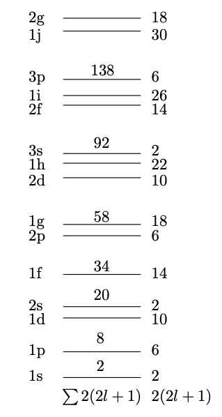
This gives us the shell structure in Fig. 3.4. Note that the levels are labelled using standard spectroscopic notation with s, p, d, f, etc. corresponding to $\mathrm{\ell }=0,1,2,3$, etc. However, the preceding index, $n$, does not correspond to the principal quantum number (as it does for electronic levels) but rather it simply labels the levels with a particular value of $\mathrm{\ell }$, beginning with the lowest energy state. Satisfyingly the ‘magic numbers’ 2, 8, and 20 emerge, but the larger ones are not reproduced. Is this due to the crude approximation of an infinite potential?

Tip 3.2.1.

Remember the spectroscopic notation for the first few angular momentum quantum numbers $\mathrm{\ell }$. There are s ($\mathrm{\ell }=0$), p ($\mathrm{\ell }=1$), d ($\mathrm{\ell }=2$), f ($\mathrm{\ell }=3$).

We can use a more realistic potential, with a finite depth and a smooth, rather than a sharp edge, as shown in Fig. 3.5. For the following values for the constants $V_0=50$ MeV, $R=1.25A^{1/3}$ fm, $a=0.524$ fm, a new energy level structure is obtained, as shown in Fig. 3.6.

Figure 3.5: Realistic potential for nuclear shell model.

Figure 3.6: Energy levels for potential in Fig 3.5.

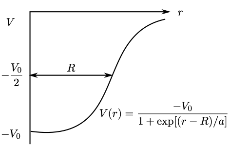
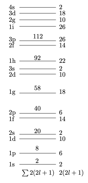
Disappointingly, we still don’t reproduce the larger magic numbers. The model we have chosen for the nuclear potential is not to blame – it’s actually quite a good representation.

3.3 Spin-orbit potential

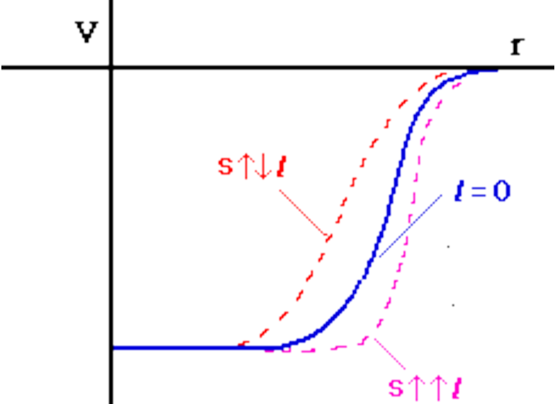
In 1949, it was shown that the addition of a spin-orbit potential could give the proper separation of the subshells. Recall that nucleons are spin 1/2 particles. The spin-orbit potential gives a correction to the usual nuclear potential depending if the spin of the nucleon is parallel or anti-parallel to its angular momentum. This is illustrated in Fig. 3.7.

Figure 3.7: The spin-orbit correction to the nuclear potential. The potential depends if the spin of the nucleon is parallel or anti-parallel to its angular momentum.

The spin-orbit potential is given by

$$V_{\mathrm{so}}(r)𝐥\cdot 𝐬.$$ (3.11)

The first term indicates this also has a radial dependence (the exact form won’t be important to us though). We will now find the expectation value of this quantity to find the resulting shift in energy levels. To do this let us first rewrite it in an easier to use form.

We can label the nuclear states (as we do in atomic physics) with the total angular momentum:

$$𝐣=𝐥+𝐬.$$ (3.12)

A single nucleon has $s=1/2$ so possible values of the total angular momentum quantum number $j$ are $\mathrm{\ell }+1/2$ or $\mathrm{\ell }-1/2$ (except for $\mathrm{\ell }=0$, when there is only a $s=1/2$ state). We can find the expectation value of $𝐥\cdot 𝐬$ as follows:

${𝐣}^2$ $=$ ${(𝐥+𝐬)}^2={𝐥}^2+2𝐥\cdot 𝐬+{𝐬}^2,$ (3.13)

$𝐥\cdot 𝐬$ $=$ ${\displaystyle \frac{1}{2}}\left({𝐣}^2-{𝐥}^2-{𝐬}^2\right).$

Recall from QM the expectation value of the operator ${𝐥}^2$ for systems involving a central potential of the form $V=V(r)$,

$$⟨{𝐥}^2⟩=\mathrm{\ell }(\mathrm{\ell }+1){\mathrm{\hslash }}^2.$$ (3.14)

Therefore we have

$$⟨𝐥\cdot 𝐬⟩=\frac{1}{2}\left[j(j+1)-\mathrm{\ell }(\mathrm{\ell }+1)-s(s+1)\right]{\mathrm{\hslash }}^2.$$ (3.15)

Example 3.3.1 (Magnetic Moment).

Question: The total magnetic moment operator $𝝁$ for a single nucleon is given by

$$𝝁={\mu }_{\mathrm{N}}\left[g_{\mathrm{\ell }}𝒍+g_{\mathrm{s}}𝒔\right]/\mathrm{\hslash },$$

where ${\mu }_{\mathrm{N}}=e\mathrm{\hslash }/(2m_{\mathrm{p}})$ is the nuclear magnetron, $g_{\mathrm{\ell }}$ and $g_{\mathrm{s}}$ are the orbital angular momentum and spin g-factors, $𝒍$ the orbital angular momentum operator and $𝒔$ the spin angular momentum operator. Calculate the expectation value of the scalar product

$$⟨𝝁\cdot 𝒋⟩.$$

Solution.

Given:

$$𝐣=𝐥+𝐬,$$ (3.16)

we need to calculate the expectation value:

$$⟨𝝁\cdot 𝐣⟩={\mu }_{\mathrm{N}}\left[g_{\mathrm{\ell }}⟨𝐥\cdot 𝐣⟩+g_{\mathrm{s}}⟨𝐬\cdot 𝐣⟩\right]/\mathrm{\hslash }.$$ (3.17)

Since

$$𝐥\cdot 𝐣=𝐥\cdot 𝐥+𝐥\cdot 𝐬,$$ (3.18)

using (3.13) gives

$$𝐥\cdot 𝐣=\frac{1}{2}\left({𝐣}^2+{𝐥}^2-{𝐬}^2\right).$$ (3.19)

The expectation value is then

$$⟨𝐥\cdot 𝐣⟩=\frac{1}{2}\left[j(j+1)+\mathrm{\ell }(\mathrm{\ell }+1)-s(s+1)\right]{\mathrm{\hslash }}^2.$$ (3.20)

Similarly (3.13) gives

$$𝐬\cdot 𝐣=\frac{1}{2}\left({𝐣}^2+{𝐬}^2-{𝐥}^2\right),$$ (3.21)

which gives the expectation value

$$⟨𝐬\cdot 𝐣⟩=\frac{1}{2}\left[j(j+1)+s(s+1)-\mathrm{\ell }(\mathrm{\ell }+1)\right]{\mathrm{\hslash }}^2.$$ (3.22)

These gives the result

$$⟨𝝁\cdot 𝐣⟩=\frac{{\mu }_{\mathrm{N}}\mathrm{\hslash }}{2}\left[\left(g_{\mathrm{\ell }}+g_{\mathrm{s}}\right)j(j+1)+\left(g_{\mathrm{\ell }}-g_{\mathrm{s}}\right)\mathrm{\ell }(\mathrm{\ell }+1)+\left(g_{\mathrm{s}}-g_{\mathrm{\ell }}\right)s(s+1)\right].$$ (3.23)

∎

Difficult 3.3.1.

Quantum numbers are always positive. For example, for a particle with spin 1/2, $s=1/2$ whether it is spin up or spin down (it is not $s=-1/2$). The $\pm$ is associated with the z-component $m_s=\pm 1/2$ states.

3.3.1 Energy splitting

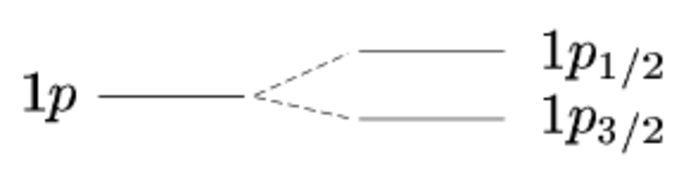
The resulting change in energy is proportional to $𝐥\cdot 𝐬$, and so depends on the orientation of nucleon spin and angular momentum. More specifically, the energy levels are split into $j=\mathrm{\ell }\pm 1/2$ levels (i.e. depending on whether the spin is parallel to angular momentum, $j=\mathrm{\ell }+1/2$, or anti-parallel, $j=\mathrm{\ell }-1/2$). We therefore label the states with an additional subscript corresponding to the $j$ value. An example is shown in Fig. 3.8 for the $1p$ level. The original $p$ level with $\mathrm{\ell }=1$ is split into $j=1/2$ and $j=3/2$ levels.

Figure 3.8: Splitting of the $1p$ level to $1p_{1/2}$ and $1p_{3/2}$ levels.

Recall that previously the degeneracy of each $\mathrm{\ell }$ level was $2(2\mathrm{\ell }+1)$. After splitting, each $j$ level has a degeneracy of $2j+1$ (there is no factor of 2 out the front since there is a single spin state for each particular $j$). You can check that the number of states is the same after and before splitting

$$2(\mathrm{\ell }+1/2)+1+2(\mathrm{\ell }-1/2)+1=2(2\mathrm{\ell }+1).$$ (3.24)

Example 3.3.2 (Spin Orbital Potential).

Calculate the energy splitting for the 1f level and then generalise this to any level.

Solution.

This has $\mathrm{\ell }=3$ with the degeneracy $2(2\mathrm{\ell }+1)=14$. The possible values of $j$ are 5/2 and 7/2 (see above) so we can label the 1f levels as $1f_{5/2}$ and $1f_{7/2}$ with degeneracies of $2j+1$, i.e. 6 and 8, respectively. This energy splitting gap between this spin-orbit pair (doublet) is proportional to the difference in $𝐥\cdot 𝐬$ (see Eqn. 3.11),

$${⟨𝐥\cdot 𝐬⟩}_{j=7/2}-{⟨𝐥\cdot 𝐬⟩}_{j=5/2}=\frac{7}{2}{\mathrm{\hslash }}^2,$$ (3.25)

or more generally

$${⟨𝐥\cdot 𝐬⟩}_{j=\mathrm{\ell }+1/2}-{⟨𝐥\cdot 𝐬⟩}_{j=\mathrm{\ell }-1/2}=\frac{1}{2}(2\mathrm{\ell }+1){\mathrm{\hslash }}^2.$$ (3.26)

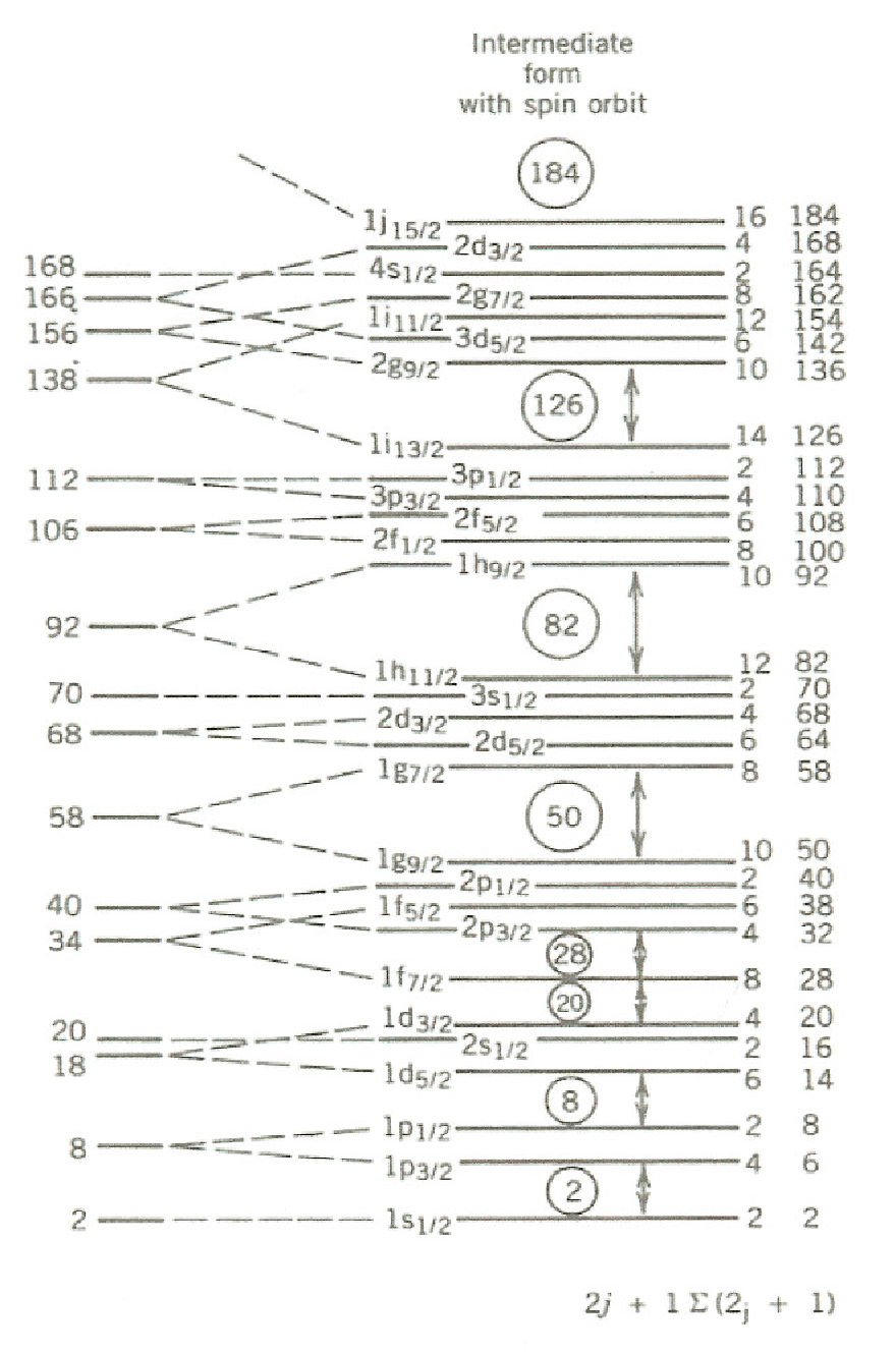
Note that the energy splitting increases with $\mathrm{\ell }$. If we choose $V_{\mathrm{so}}(r)$ to be negative then the $1{\mathrm{f}}_{7/2}$ level is pushed down into the gap between the second and third shells, increasing the capacity of the third shell from 20 to the magic number of 28 (see Fig. 3.9). In a similar way, all the magic numbers are accounted for.

Including an appropriate radial dependence for the $V_{\mathrm{so}}(r)$ term, we obtain the shell structure shown in Fig. 3.9, where it can be seen that all the magic numbers are reproduced.

Figure 3.9: Energy levels including the effect of spin-orbit coupling. The number to the right now shows the degeneracy of each of $j$ level, which is $2j+1$.

3.3.2 Filling of shells

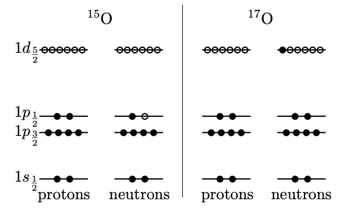
With the shell model in hand, we can now write down the structure of particular nuclei. To fill shells, we first work out the number of protons and neutrons, and add them according to the next available lowest energy state of Fig. 3.9. Fig. 3.10 shows examples of filling shells for ¹⁵O and ¹⁷O. Note that protons and neutrons are not identical particles so have different quantum numbers and fill separate sets of energy levels.

Figure 3.10: Filling shells in ¹⁵O and ¹⁷O.

3.4 Exercises

Example 3.4.1 (Shell Filling).

In a particular version of the shell model with a single valence nucleon (the nucleon outside a filled shell), the nuclear spin is equal to the total angular momentum of the valence nucleon. Give the filling of shells for protons and neutrons and hence determine the nuclear spin for

1. ${}_3{}^7\mathrm{Li}$

2. ${}_6{}^{15}\mathrm{C}$

3. ${}_9{}^{17}\mathrm{F}$

Solution.

1. The configurations are given by:

2. Protons: ${(1s_{1/2})}^2{(1p_{3/2})}^1$, neutrons: ${(1s_{1/2})}^2{(1p_{3/2})}^2$. The valence nucleon is a proton and hence the nuclear spin is 3/2.

3. Protons: ${(1s_{1/2})}^2{(1p_{3/2})}^4$, neutrons: ${(1s_{1/2})}^2{(1p_{3/2})}^4{(1p_{1/2})}^2{(1d_{5/2})}^1$. The valence nucleon is a neutron and hence the nuclear spin is 5/2.

4. Protons: ${(1s_{1/2})}^2{(1p_{3/2})}^4{(1p_{1/2})}^2{(1d_{5/2})}^1$, neutrons: ${(1s_{1/2})}^2{(1p_{3/2})}^4{(1p_{1/2})}^2$. The valence nucleon is a proton and hence the nuclear spin is 5/2.